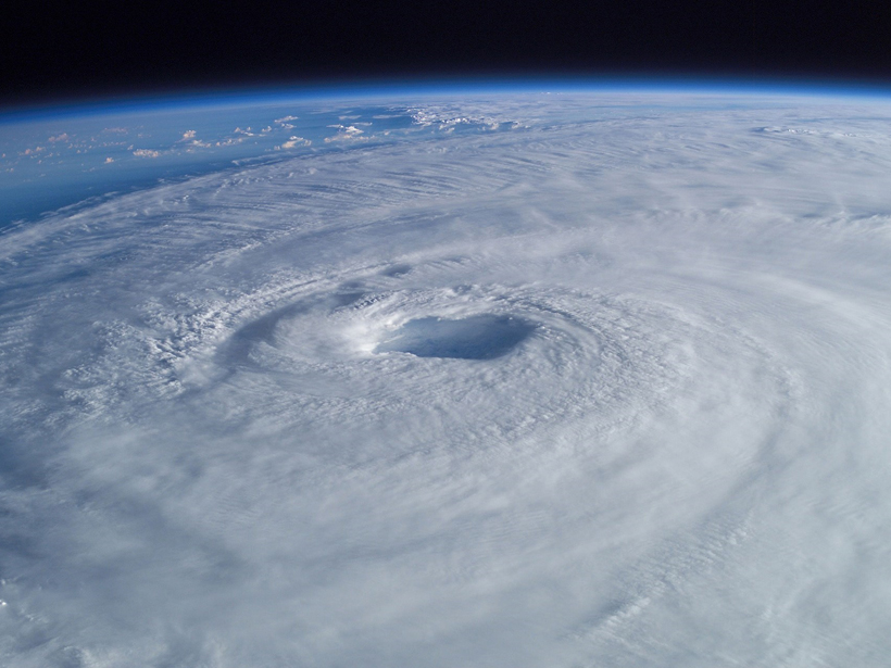
A fascinating aspect of the climate system is that its variability is governed by some simple mathematical relationships. A recent paper in Reviews of Geophysics discusses how these mathematical relationships—in the form of power-laws—structure a large part of climate variability in terms of time, space, and intensity. Understanding how climate variability is structured helps us to make robust climate reconstructions and skillful future predictions. Here, two authors provide a brief overview on what a power-law is, how it can be used to improve our understanding of the climate system, and the physical mechanisms behind it.
How are different aspects of the climate system interrelated?
Climate variables—such as temperature, precipitation, total ozone, relative humidity, and sea level change—are strongly interconnected, both over long durations of time and across large spatial distances. This can be seen in datasets: there are correlations in data averages over long intervals or between distant areas.
The majority of correlations in climate can be described by a simple mathematical relationship called “scaling.”
A neat finding is that the majority of correlations in climate can be described by a simple mathematical relationship called “scaling,” which says that averages on different scales are related by a simple mathematical function—a power law.
In practice this means that, for example, the duration of temperature fluctuations increases systematically, as the temperature fluctuation grows larger.
Furthermore, the likelihood of an event to happen is also found to decrease the more intense the event is. This is similar to the Richter law for earthquakes, which says that small earthquakes happen very often while very big earthquakes occur rarely.

How can mathematical tools be applied to understand these relationships?
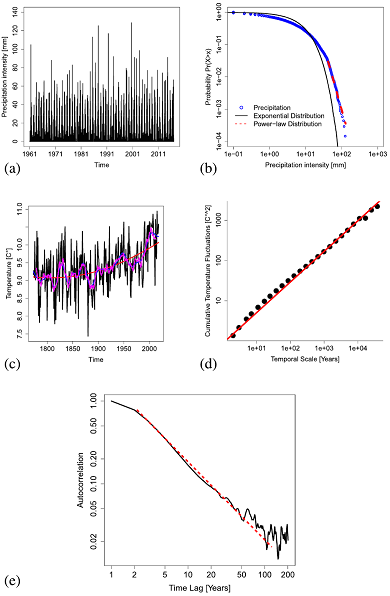
Power-laws appear as straight lines in plots where both axes have a logarithm scaling, and the slopes indicate the scaling exponents. They are familiar to many scientists from undergraduate physics classes.
One well known example is the relationship between a pendulum’s angular frequency and its length: the angular frequency is proportional to the inverse square root of the length.
Another example is how the gravitational force between two bodies depends on their distance from one another: the gravitational force is proportional to the inverse distance squared.
It is fascinating that power laws also exist in climate time series, as shown in the charts to the right, where the scaling exponents measure the persistence of climate anomalies and the likelihood of extreme events of different intensity.
Which climate variables display scaling behavior?
Scaling behavior is ubiquitous in the climate system. It has been detected in many climate variables, using observational in-situ records, paleo-reconstructions, and model simulations.
The most prominent is surface air temperature, where the most pronounced scaling behavior is found in the ocean and coastal regions, as shown in the map below. However, other variables—such as precipitation, river runoff, ozone levels, humidity, and sea level height—also have this property, suggesting that scaling is a very widespread characteristic of the climate system.
What are the physical mechanisms behind scaling?
There are a few possible explanations for scaling in the climate system, all caused by the underlying nonlinear nature of the equations of motion. A prime example is turbulence: the scaling behavior in which energy is distributed among spatial scales was discovered by A. N. Kolmogorov in 1941.
Temporal scaling can be explained due to the nonlinear nature of the equations governing the climate system and the interaction of components of the climate system with different time scales such as the atmosphere (whose typical timescale is from seconds to weeks), the ocean (with time scales of weeks to decades), and ice sheets (changing on time scales of decades to millennia).
How can scaling be applied to improve climate modeling and prediction?
Using scaling enables us to faster compute the response of the Earth system to greenhouse gas emissions, and to improve our understanding of predictability and climate models. Recently, a Stochastic Seasonal to Inter-Annual Prediction System has been developed from this perspective. Its forecast accuracy compares favorably with operational long-range forecasting models based on traditional climate models.
What are some of the unresolved questions where additional research, data or modeling is needed?
Through scaling analysis, we have now a better understanding of the climate system and appreciate that it consists of different time scales characterized by different scaling relationships. While for weather (up to 2 weeks) and climate (more than 30 years) timescales, the variability strongly increases with time scale; this is not the case for the timescales in between (2 weeks to 30 years) where the increase is rather weak. How this affects predictability on these time scales is an open question. It is worth noting that an inclusion of the scaling behaviors in traditional climate models may be also helpful (for example, for the improvement of subgrid-scale parameterizations), but more efforts are still required in this regard.
How well scaling can contribute to the reconstruction of past climate is another ongoing area of research. Scaling of paleoclimate data has received a lot of attention and has been used in evaluating how well climate models reproduce observed long-term climate variability. While global mean temperature variability on interannual to millennial time scales seems to be consistent between climate models and climate reconstructions, the strong discrepancy of slow climate variability at regional scales calls for continued research on the temporal and spatial structures of climate variability and also on improving the interpretation and quality of paleo-climate records. The PAGES group “Climate Variability across Scales” is currently working on this issue.
A better appreciation of how scaling links climate variability on different scales has already improved our understanding of the climate system, but there is still much exciting theoretical and applied work to be done in this field.
—Christian L. E. Franzke ([email protected]; ![]() 0000-0003-4111-1228), University of Hamburg, Germany; and Naiming Yuan (
0000-0003-4111-1228), University of Hamburg, Germany; and Naiming Yuan (![]() 0000-0003-0580-609X), Institute of Atmospheric Physics, Chinese Academy of Sciences, China
0000-0003-0580-609X), Institute of Atmospheric Physics, Chinese Academy of Sciences, China
Citation:
Franzke, C. L. E.,Yuan, N. (2020), Is climate variability organized?, Eos, 101, https://doi.org/10.1029/2020EO145366. Published on 11 June 2020.
Text © 2020. The authors. CC BY-NC-ND 3.0
Except where otherwise noted, images are subject to copyright. Any reuse without express permission from the copyright owner is prohibited.