
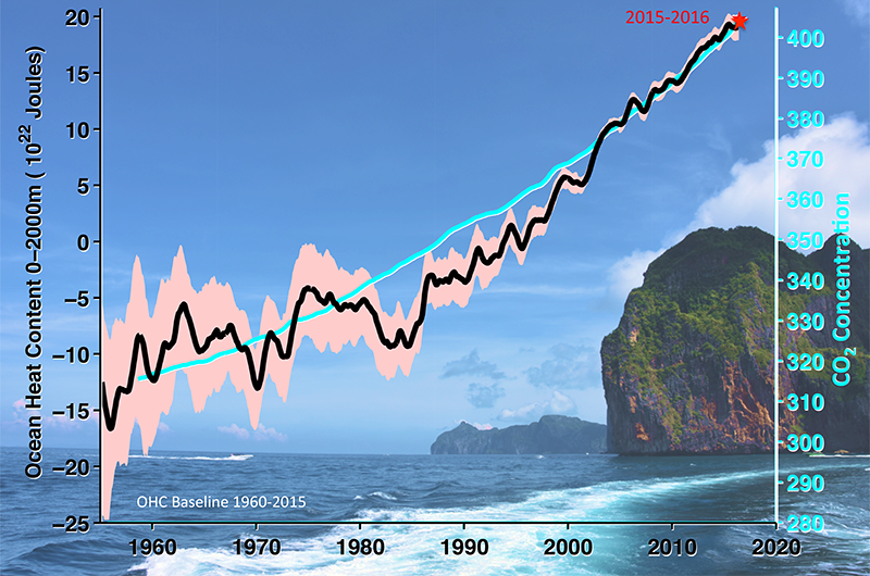
Humans have released carbon dioxide and other greenhouse gases in sufficient quantity to change the composition of the atmosphere (Figure 1). The result is an accumulation of heat in Earth’s system, commonly referred to as global warming. Earth’s climate has responded to this influx of heat through higher temperatures in the atmosphere, land, and ocean. This warming, in turn, has melted ice, raised sea levels, and increased the frequency of extreme weather events: heat waves and heavy rains, for example. The results of these weather events include wildfires and flooding, among other things [Intergovernmental Panel on Climate Change, 2013].
Decision-makers, scientists, and the general public are faced with critical questions: How fast is Earth’s system accumulating heat, and how much will it warm in the future as human activities continue to emit greenhouse gases?
Ocean heating and sea level rise show stronger evidence that the planet is warming than does global average surface temperature, which relies on air temperature measurements.
Here we explore better ways of measuring global warming to answer these questions. Natural temperature variability is much more muted in the ocean than in the atmosphere, owing to the ocean’s greater ability to absorb heat (its heat capacity). As a result, ocean heating and sea level rise, which are measured independently, show stronger evidence that the planet is warming than does global average surface temperature, which relies on air temperature measurements. In other words, these ocean measurements could provide vital signs for the health of the planet.
Thus, we suggest that scientists and modelers who seek global warming signals should track how much heat the ocean is storing at any given time, termed global ocean heat content (OHC), as well as sea level rise (SLR). Similar to SLR, OHC has a very high signal-to-noise ratio; that is, it clearly shows the effects of climate change distinct from natural variability.
Why Do Changes in Surface Temperatures Obscure Signals from Global Warming?
To determine how fast Earth’s systems are accumulating heat, scientists focus on Earth’s energy imbalance (EEI): the difference between incoming solar radiation and outgoing longwave (thermal) radiation. Increases in the EEI are directly attributable to human activities that increase carbon dioxide and other greenhouse gases in the atmosphere [e.g., Trenberth et al., 2014].
The most visible sign of a warming climate is the increase in air temperature, which affects the climate and weather patterns. Changes in climate and weather affect the viability of plants and animals and our food and water supplies.
Monthly averages of global mean surface temperature (GMST) include natural variability, and they are influenced by the differing heat capacities of the oceans and land masses. Causes of natural variability include forcings that are external to the climate system (e.g., volcanic eruptions and aerosols and the 11-year sunspot cycle) and internal fluctuations (weather phenomena, monsoons, El Niño/La Niña, and decadal cycles).
All of these fluctuations make it difficult to extract the signal from noise in the measurements. But the oceans tell a different story.
What Global Warming Signals Can Be Found in the Oceans?
Scientists have long known that the extra heat trapped by increasing greenhouse gases mainly ends up in the oceans (more than 90%) [Rhein et al., 2013]. Hence, to measure global warming, we have to measure ocean warming.
The oceans present myriad challenges for adequate monitoring. To take the ocean’s temperature, it is necessary to use enough sensors at enough locations and at sufficient depths to track changes throughout the entire ocean. It is essential to have measurements that go back many years and that will continue into the future.
Since 2006, the Argo program of autonomous profiling floats has provided near-global coverage of the upper 2,000 meters of the ocean over all seasons [Riser et al., 2016]. In addition, climate scientists have been able to quantify the ocean temperature changes back to 1960 on the basis of the much sparser historical instrument record [Cheng et al., 2017].
The increase in ocean heat content observed since 1992 in the upper 2,000 meters is about 2,000 times the total net generation of electricity by U.S. utility companies in the past decade.
From these temperature measurements, scientists extract OHC. These analyses show that during 2015 and 2016, the heat stored in the upper 2,000 meters of the world ocean reached a new 57-year record high (Figure 1). This heat storage amounts to an increase of 30.4 × 10²² Joules (J) since 1960 [Cheng et al., 2017], equal to a heating rate of 0.33 Watts per square meter (W m−2) averaged over Earth’s entire surface—0.61 W m−2 after 1992. Improved measurements have revised these values upward by 13% compared with the results of the Fifth Assessment Report of the Intergovernmental Panel on Climate Change [Rhein et al., 2013]. For comparison, the increase in OHC observed since 1992 in the upper 2,000 meters is about 2,000 times the total net generation of electricity by U.S. utility companies in the past decade [U.S. Energy Information Administration, 2016].
But what about heat capacity over the full ocean depth? The answer requires a bit more calculation. Any increase in heat contributes to the thermal expansion of seawater and, consequently, SLR [Church et al., 2013]. Any energy added in Earth’s system also causes land-based ice to melt, further contributing to SLR by adding water to the ocean.
Studies show that taking the full ocean depth, ice melt, and other factors into account, Earth is estimated to have gained 0.40 ± 0.09 W m−2 since 1960 and 0.72 W m−2 since 1992 [Cheng et al., 2017]—18% higher than for the top 2,000-meter OHC alone.
Human-Caused Warming or Just Natural Variations?
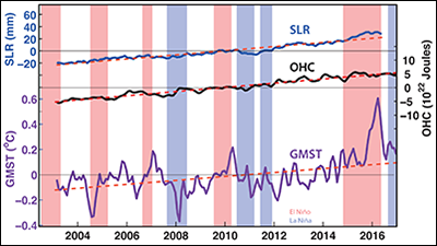
The amplitude of the global warming signature (signal) compared with natural variability (noise) defines how well a metric tracks global warming. The “noise level,” that is, the amplitude of internal variability, approximated here by the standard deviation (σ) of the OHC time series after the linear trend is removed, amounts to 0.77 × 10²² J from 2004 to 2015 (Table 1). The linear trend of OHC is 0.79 ±0.03 × 10²² J year−1 within the same period (Figure 2).
Table 1. The Linear Trend (with 95% Confidence Level) for the Three Key Climate Indicators: Global Mean Surface Temperature (GMST), Ocean Heat Content (OHC), and Sea Level Rise (SLR)a
| Linear Trend | σ | S/N (1/years) | Time (years) | |
| GMST | 0.016°C ± 0.005°C/yr | 0.110°C/yr | 0.14 | 27 |
| OHC | 0.79 ± 0.03 × 10²² J/yr | 0.77 × 10²² J/yr | 1.03 | 3.9 |
| SLR | 3.38 ± 0.10 mm/yr | 3.90 mm/yr | 0.87 | 4.6 |
aAlso shown are the corresponding noise levels (standard deviation σ), signal-to-noise ratio (S/N), and the time in years required to detect a trend (approximately the time when the linear trend exceeds 4 times the interannual standard deviation). All values are for 2004–2015. Units: yr = year, J = joules, mm = millimeters.
So what time interval is needed to detect a trend given the noise within this time series? Working backward, the signal showing OHC increase, averaged over only 3.9 years, typically exceeds the noise at the 95% confidence level (outside ±2σ error bars; Table 1). Thus, it is relatively straightforward to detect a long-term trend in OHC.
For the GMST record, the trend is 0.016°C ± 0.005°C per year for 2004–2015, and σ of the detrended GMST time series is 0.110°C (Table 1). These values and Figure 2 show that the noise is much larger than the signal. Thus, to detect a warming trend in the GMST record that exceeds a ±2σ noise level, scientists need at least 27 years of data.
Satellite altimetry has provided global observations of rising sea levels since the early 1990s [Cazenave et al., 2014]. The linear trend of global mean SLR from 2004 to 2015 amounts to 3.38 ± 0.10 millimeters per year, and the σ of the detrended global mean is 3.90 millimeters (Table 1). Thus, 4.6 years are sufficient to detect a robust upward trend in SLR: a signal-to-noise ratio approximately 6 times larger than for GMST.
OHC and SLR Are Robust Indicators of Global Warming
A comparison of the changes and fluctuations in the three observational climate indicators (SLR, OHC, and GMST; Figure 2) clearly shows that both OHC and SLR are much better indicators of global warming than GMST. These two measures are related but also sufficiently different and independently measured to both be of interest.
The large fluctuations in GMST and its sensitivity to natural variability mean that using this measurement to argue that global warming is (or is not) happening requires care. An excellent example is the 1998–2013 period, when energy was redistributed within Earth’s system and the rise of GMST slowed [Yan et al., 2016].
By contrast, the OHC and sea level increased steadily during this period, providing clear and convincing evidence that global warming continued.
The Need to Take the Pulse of the Planet
Monitoring the past and current climate helps us better understand climate change and enables future climate projections. We must maintain and extend the existing global climate observing systems [Riser et al., 2016; von Schuckmann et al., 2016] as well as develop improved coupled (ocean-atmosphere) climate assessment and prediction tools to ensure reliable and continuous monitoring for Earth’s energy imbalance, ocean heat content, and sea level rise.
The EEI has implications for the future and should be fundamental in guiding future energy policy and decisions; it is the heartbeat of the planet. Changes in OHC, the dominant measure of EEI, should be a fundamental metric along with SLR.
As we continue to scrutinize the fidelity of specific climate models, it is critical to validate their energetic imbalances as well as their depiction of GMST. The fact that the Coupled Model Intercomparison Project Phase 5 (CMIP5) ensemble mean accurately represents observed global OHC changes [Cheng et al., 2016] is critical for establishing the reliability of climate models for long-term climate change projections.
Consequently, we recommend that both the EEI and OHC be listed as output variables in the CMIP6 models, in addition to SLR and GMST. This vital sign informs societal decisions about adaptation to and mitigation of climate change [Trenberth et al., 2016].
Acknowledgments
L.C. and J.Z. were supported by XDA11010405. K.E.T. and J.F. were partially sponsored by the U.S. DOE (DE-SC0012711). The National Center for Atmospheric Research (NCAR) is sponsored by the U.S. National Science Foundation.
References
Cazenave, A., et al. (2014), The rate of sea-level rise, Nat. Clim. Change, 4(5), 358–361, https://doi.org/10.1038/nclimate2159.
Cheng, L., et al. (2016), Observed and simulated full-depth ocean heat content changes for 1970–2005, Ocean Sci., 12, 925–935, https://doi.org/10.5194/os-12-925-2016.
Cheng, L., et al. (2017), Improved estimates of ocean heat content from 1960 to 2015, Sci. Adv., 3, e1601545, https://doi.org/10.1126/sciadv.1601545.
Church, J. A., et al. (2013), Sea level change, in Climate Change 2013: The Physical Science Basis, edited by T. F. Stocker et al., Cambridge Univ. Press, Cambridge, U.K., https://doi.org/10.1017/CBO9781107415324.026.
Intergovernmental Panel on Climate Change (2013), Climate Change 2013: The Physical Science Basis, edited by T. F. Stocker et al., Cambridge Univ. Press, Cambridge, U.K., https://doi.org/10.1017/CBO9781107415324.
Rhein, M., et al. (2013), Observations: Ocean, in Climate Change 2013: The Physical Science Basis, edited by T. F. Stocker et al., Cambridge Univ. Press, Cambridge, U.K., https://doi.org/10.1017/CBO9781107415324.010.
Riser, S. C., et al. (2016), Fifteen years of ocean observations with the global Argo array, Nat. Clim. Change, 6, 145–153, https://doi.org/10.1038/nclimate2872.
Trenberth, K., J. Fasullo, and M. Balmaseda (2014), Earth’s energy imbalance, J. Clim., 27, 3129–3144, http://dx.doi.org/10.1175/JCLI-D-13-00294.1.
Trenberth, K. E., M. Marquis, and S. Zebiak (2016), The vital need for a climate information system, Nat. Clim. Change, 6, 1057–1059, https://doi.org/10.1038/nclimate3170.
U.S. Energy Information Administration (2016), Electric power annual 2015, U.S. Dep. of Energy, Washington, D. C., https://www.eia.gov/electricity/annual/html/epa_01_02.html.
von Schuckmann, K., et al. (2016), An imperative to monitor Earth’s energy imbalance, Nat. Clim. Change, 6, 138–144, https://doi.org/10.1038/nclimate2876.
Yan, X.-H., et al. (2016), The global warming hiatus: Slowdown or redistribution?, Earth’s Future, 4, 472–482, https://doi.org/10.1002/2016EF000417.
Author Information
Lijing Cheng (@Lijing_Cheng), International Center for Climate and Environment Sciences, Institute of Atmospheric Physics, Chinese Academy of Sciences, Beijing; Kevin E. Trenberth (email: [email protected]) and John Fasullo (@jfasullo), National Center for Atmospheric Research, Boulder, Colo.; John Abraham, University of St. Thomas, St. Paul, Minn.; Tim P. Boyer, National Centers for Environmental Information, National Oceanic and Atmospheric Administration, Silver Spring, Md.; Karina von Schuckmann, Mercator Océan, Ramonville St Agne, France; and Jiang Zhu, International Center for Climate and Environment Sciences, Institute of Atmospheric Physics, Chinese Academy of Sciences, Beijing
Citation:
Cheng, L.,Trenberth, K. E.,Fasullo, J.,Abraham, J.,Boyer, T. P.,von Schuckmann, K., and Zhu, J. (2017), Taking the pulse of the planet, Eos, 98, https://doi.org/10.1029/2017EO081839. Published on 13 September 2017.
Text © 2017. The authors. CC BY-NC-ND 3.0
Except where otherwise noted, images are subject to copyright. Any reuse without express permission from the copyright owner is prohibited.