
Editors’ Vox is a blog from AGU’s Publications Department.
Radiocarbon is a rare, but powerful, isotope of carbon that is used widely as a dating tool and as an environmental tracer. A recent study in Reviews of Geophysics explores the use of radiocarbon in the field of paleoceanography. We asked the authors to give an overview of how radiocarbon is used, what recent advances have been made possible by radiocarbon, and what questions remain.
What is radiocarbon and how is it used in the biogeosciences?
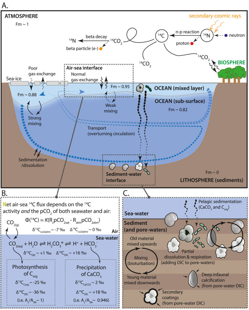
Radiocarbon is a carbon isotope with mass 14 that is produced in the atmosphere due to cosmic radiation striking nitrogen atoms. Radiocarbon is rare and unstable; it accounts for only about 1.2 x 10⁻¹⁰ percent of carbon atoms, and undergoes radioactive decay with a half-life of about 5,700 years. The total amount of radiocarbon in the Earth system depends primarily on the rate at which it is produced, which can vary due to changes in the flux of cosmic radiation into the Earth’s atmosphere.
Radiocarbon is widely used in the biogeosciences, both as a carbon cycle tracer and as a dating tool. The utility of radiocarbon derives primarily from the way it is produced in the atmosphere, and its radioactive decay. The most widely known application of radiocarbon is for ‘radiocarbon dating’, where the amount by which the radiocarbon concentration of an object, measured today in the laboratory, has decreased relative to the concentration it had when it formed. This tells us the amount of ‘decay time’ experienced by the object, and therefore its age. However, because it participates in the carbon cycle, radiocarbon can also serve as an environmental ‘tracer’ that provides a measure of carbon residence times and/or carbon exchange between carbon bearing reservoirs in the Earth system. Furthermore, as a cosmogenic nuclide, radiocarbon can also provide insights into cosmic radiation fluxes and therefore past variability in solar activity and/or the Earth’s magnetic field strength.
How does radiocarbon provide a “clock” for carbon movement in the environment?
Radiocarbon atoms are essentially atmospherically ‘tagged’ carbon atoms with a finite lifetime of about 8,267 years on average. The radiocarbon concentration (14C/C ratio) of a given Earth system reservoir, e.g. the ocean, will depend on how long it takes for its carbon pool to be exchanged (directly or indirectly) with the atmosphere, on average. For example, an atom of carbon resides in the deep ocean far longer than it does in the surface ocean, before it is replaced by a ‘new’ carbon atom from the atmosphere. Accordingly, the radiocarbon concentration of the deep ocean is about 17% less than that of the surface ocean, which represents roughly 1,500 years of additional radiocarbon decay in the deep ocean. All else being equal, a slower turnover of the ocean’s carbon pool would cause its radiocarbon concentration to decrease further, relative to the surface ocean and atmosphere.
Similar principles can be used to study the residence times of other carbon pools, such as particulate organic matter in sediments, or dissolved organic matter in seawater, etc. However, in all cases, the cycling of radiocarbon is rarely completely straightforward: it can provide unique insights on timescales for carbon cycling and exchange, but it must be treated carefully.
How is radiocarbon used in numerical models?
Numerical models, of varying complexity, can make use of radiocarbon as an additional tracer, implemented alongside stable carbon, and permitting additional insights into the timescales and processes of carbon exchange in model simulations. This can be useful for tracking impacts, such as gas-exchange or ocean transports on carbon cycling. It can also be extremely useful for comparing model outputs with observations, though only for about the last 50,000 years.
Radiocarbon is a relatively long-lived isotope (average lifetime of about 8,223 years), which means that it can be difficult to implement in more complex numerical models where the computational cost of simulating several thousands of years (as needed for the radiocarbon cycle to reach an equilibrium state) may be excessive. However, new methods are helping to circumvent these challenges, such that the application of radiocarbon as a tracer in more complex and comprehensive Earth system models is likely to expand.
Why is radiocarbon such a powerful tool in the field of paleoceanography?
In the right circumstances, radiocarbon can serve as a uniquely useful dating tool in paleoceanography, allowing accurate dates for carbon-bearing marine sedimentary components back to about 50,000 years. For this application, the principal challenge is knowing how to ‘calibrate’ a calculated radiocarbon age, so as to correct for past changes in the radiocarbon production rate and past changes in radiocarbon cycling within the Earth system. Currently, we only possess a good calibration curve for the atmosphere, and the principal challenge for marine radiocarbon dating arises from the need to correct for ocean-atmosphere radiocarbon offsets, or so-called ‘marine reservoir age’ offsets.
An alternative application of marine radiocarbon measurements turns this situation on its head, and uses independent dating constraints to investigate past changes in radiocarbon production and cycling instead. This can provide uniquely useful insights into past changes in the carbon cycle, solar activity, or the Earth’s magnetic field strength.

What have been some exciting recent developments or discoveries?
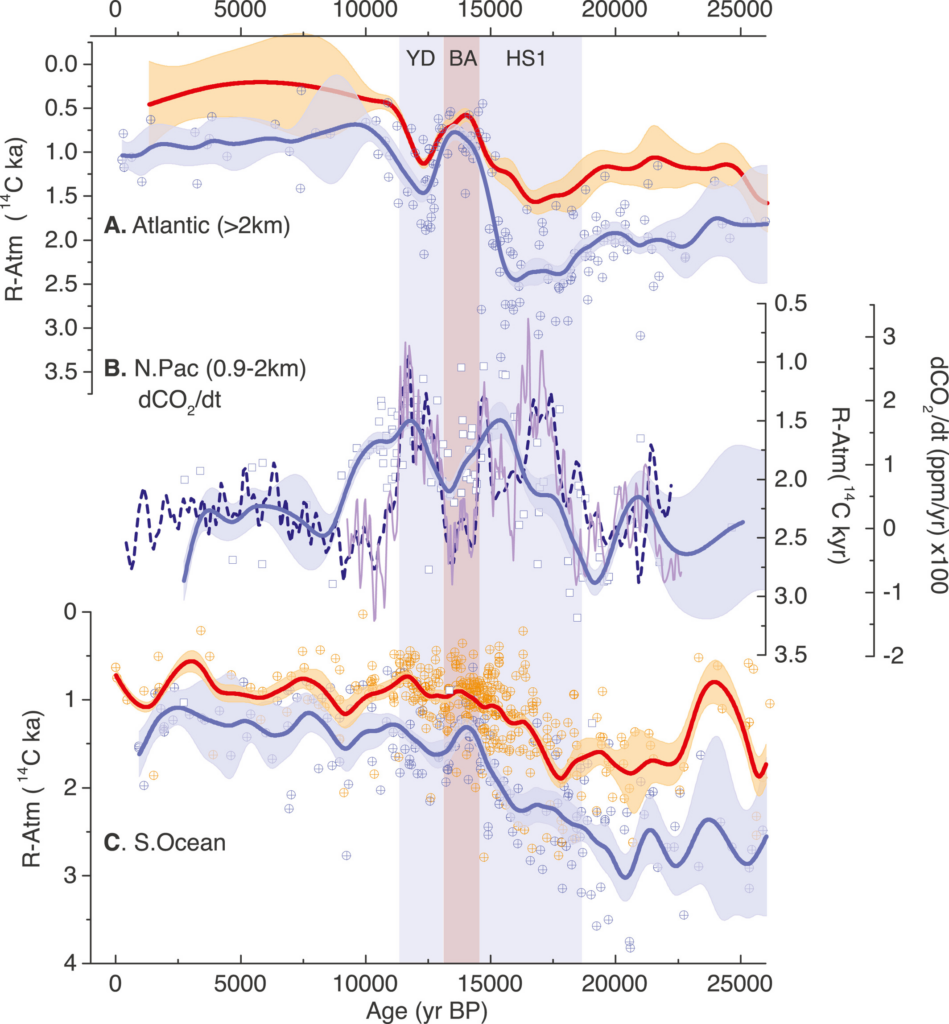
Radiocarbon has been used to investigate marine carbon cycle changes for decades, building to a large extent on the pioneering work of Wally Broecker. One exciting development, due to the collective efforts of many people over many years, is the recent emergence of a reasonably clear picture of how the distribution of radiocarbon in the ocean interior has evolved over the last 25,000 years in association with global and regional climate changes. The compiled data show that:
- the ocean’s radiocarbon concentration was on average lower at the Last Glacial Maximum than for the pre-industrial, by the equivalent of several hundred years of radiocarbon decay;
- the ‘rejuvenation’ of the ocean interior occurred in a series of steps that were linked with regional climate anomalies (i.e. the so-called ‘bipolar seesaw’), which involved the alternating predominance of the three key high-latitude regions of ocean-atmosphere heat and carbon exchange (North Atlantic, Southern Ocean and North Pacific);
- the bulk of the reconstructed changes in ocean-atmosphere radiocarbon age offsets for the deep ocean appear to have occurred prior to the approximate mid-point of the last deglaciation (about 15,000 years ago).
The picture of deglacial radiocarbon cycling that has now come into focus underlines the importance of the Southern Ocean and North Pacific as key regulators of ocean-atmosphere carbon/radiocarbon exchange, which operate in coordination with perturbations to the Atlantic Meridional Overturning Circulation (AMOC). At the same time, the collected data raise new questions regarding the mechanistic link between deep ocean ‘ventilation’ and atmospheric CO2. To some extent, the latter may depend on a more explicit characterization of the link between ocean ‘ventilation’ (as defined above) and evolving ocean-atmosphere radiocarbon disequilibrium.
What are some of the unresolved questions where additional research, data, or modeling are needed?
One interesting question that has emerged, in light of a handful of puzzling radiocarbon datasets, relates to the significance of sedimentary and/or volcanic/metamorphic carbon fluxes to the deep ocean, and how these may have varied on millennial or glacial-interglacial timescales to affect the radiocarbon cycle. While the balance of evidence appears to rule out an overwhelming input of ‘geological’ carbon to the ocean across the last deglaciation, the question remains an important one to fully clarify and quantify.
Another exciting and unresolved question bears on the role of ocean ‘ventilation’ (i.e. the combined effects of air-sea gas exchange and overturning) in centennial jumps in atmospheric CO2, which have only recently been identified in new high-resolution ice-core records. Tantalizing, if highly tentative, radiocarbon evidence suggests a role for ocean ventilation in these abrupt CO2 jumps, but the picture remains far from clear.
Further, one of the main impediments to accurate radiocarbon dating in paleoceanography currently derives from uncertainty in the ‘marine reservoir age’ corrections that should be applied to marine radiocarbon dates prior to calibration using the only available (atmospheric) calibration curve. A key area for future work will be to improve our understanding of temporal and spatial marine reservoir age variability in the past. Due to the complexity of the problem, this emerges as a ‘grand challenge’ that amounts to understanding the evolving closure of the global radiocarbon cycle across the last glacial cycle.
—Luke C. Skinner ([email protected];  0000-0002-5050-0244), University of Cambridge, United Kingdom; and Edouard Bard (0000-0002-7237-8622), College de France & CEREGE, France
Editor’s Note: It is the policy of AGU Publications to invite the authors of articles published in Reviews of Geophysics to write a summary for Eos Editors’ Vox.