In the Arctic regions, marine transport operations, tourism businesses, resource extraction operations, and local communities rely on accurate reporting and forecasting of sea ice conditions. For example, recently, several coastal communities experienced critical shortages of heating fuel and gasoline during the winter months because an unforeseen early freeze-up cut short barge delivery of fuel.
Arctic sea ice reaches its maximum extent each March and its minimum extent each September. In addition to the yearly trends, routine satellite monitoring of polar regions has documented a decline in total Arctic sea ice extent since 1979. The largest and most widespread losses, which occur in September, affect an area as large as Ireland (a loss of 86,000 square kilometers per year, or 13.3% per decade).
The eight lowest September sea ice extents have all occurred within the past 8 years. As a result, Arctic resource extraction and ship traffic have increased [Pizzolato et al., 2014], leading to growing interest in developing reliable methods to predict the summer minimum sea ice extent a few months in advance.
Starting in 2008, the Study of Environmental Change (SEARCH) program began collecting, from the sea ice forecasting community, summertime estimates of the upcoming September Arctic sea ice extent and synthesizing them in monthly reports called the Sea Ice Outlook (SIO). Contributors to the reports use a wide variety of methods to generate their estimates, including heuristic forecasts, statistical and/or dynamical models, ice-ocean coupled models, and fully coupled ice-ocean-atmospheric models.
Results from the SIO are shared with other researchers and interested members of the general public through the Arctic Research Consortium of the United States.
Interest in the SIO is substantial, with more than 192,740 unique views since the outlook began. In 2013, a newly funded interagency project, the Sea Ice Prediction Network (SIPN), took over SEARCH’s synthesis effort.
The Need for Forecasts of Sea Ice Conditions
Information on ice conditions is extremely important to local communities and industries. Because of this, spatial maps on the probability of timing of ice-free conditions provided in the 2014 SIO were an important addition to the standard pan-Arctic sea ice extent forecasts originally solicited by for SIO. In 2015, SIPN will consider adding additional metrics, such as the timing of ice breakup, freeze-up, and thickness.

Shipping and hydrocarbon industries in Alaskan and Canadian waters are particularly interested in improved sea ice information and predictions over several time scales. For example, barge and vessel traffic and oil fields on the North Slope rely on forecasts of ice conditions and potential hazards on synoptic time scales (a few days to a week), as they are relevant to ice closing in toward the coast.
Shipping and hydrocarbon industries in Alaskan and Canadian waters are particularly interested in improved sea ice information and predictions.
Variations in the distribution of ice thickness and perennial ice—ice remaining from previous years—are hazards of particular concern, requiring forecasts at the onset of the operational season as well as synoptic and subseasonal forecasts over the course of the season. Seasonal predictions of breakup, freeze-up, and overall ice regimes provide an overview for conditions lasting several months. The need for ice thickness assessments, multiyear-ice assessments, and seasonal-scale forecasts dovetails with data needs for initialization and validation of predictions based on coupled ice-ocean and ice-ocean-atmosphere models.
Stakeholders in coastal communities place a high priority on improved predictions of fall freeze-up at the seasonal to submonthly scale. The presence of sea ice in the fall is a key constraint for a range of activities, including resupplying northern communities. Sea ice also affects potential hazards such as the exposure of coastlines to fall storms.
Searching for Meaningful Diagnostics
In April 2014, SIPN hosted its first sea ice prediction workshop. Scientists from around the world attended, with representation from the modeling and observation communities, as well as operational forecast centers. These scientists put forward several recommendations to improve predictions. They placed the highest priority on model intercomparison projects, improvements in ice thickness data retrieval, and assimilation of observations into models.
The need for more-sophisticated diagnostics was a recurring theme in the discussions. For the first few years of the SIO, ice extent was almost exclusively the only metric considered, yet it is clear that such a spatially integrated metric is of little use to most stakeholders.

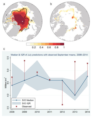
Five groups responded to a 2014 request for submissions of spatial predictions of the date of ice loss and the probability that September sea ice concentration (the fraction of a given area that is covered by ice) will be greater than 15%. Although these results show varying degrees of skill in capturing the ice edge location (Figure 1a), the multimodel mean yields a more skillful outlook than any individual dynamical model, a feature also seen in other climate forecasts [e.g., Krishnamurti et al., 1999].
General agreement across models shows that the most unpredictable feature of the September 2014 ice cover was the significant loss of ice in the Laptev Sea and the above-average ice cover in the Barents Sea (Figure 1b). It is telling that these are the regions within the Arctic where summer atmospheric forcing was most extreme, with warm southerly winds over the Laptev Sea and cold northerly winds over the Barents Sea. Because the atmosphere is mostly unpredictable beyond 1 or 2 weeks, the sea ice forecasts initialized in late spring may not be able to accurately predict sea ice features that develop as a result of extreme summer atmospheric conditions.
Which Models Are Most Accurate?
We evaluated SIO contributions from 2008 to 2013 and found that median predictions tended to be accurate in years when the extent followed the long-term accelerating trend [Stroeve el al., 2014]. For example, the observed September 2014 extent was 100,000 square kilometers less than that observed in 2013, and the median of the current sea ice extent estimations in the SIO is closer to the observed sea ice extent than the median for contributions in 2013 (Figure 1c).
In 2014, about one third of contributions came from dynamical climate models that, as a multimodel ensemble, bracketed the observed value for each month the forecasts were issued. These forecasts were more accurate for start dates closer to September, that is, when the models were initialized using the most recent observations.
An analysis of the differences between predicted and observed sea ice extents using various methods suggests that the SIO forecasts capture accelerating rates of ice loss better than a linear trend approach, although only slightly better.
Limitations of Predictability
Given inherent uncertainties, what are the limits that determine how well any predictive model can perform? Several studies have used a “perfect model” approach to estimate the limit of Arctic sea ice predictability. These idealized prediction studies suggest that skillful forecasts for monthly pan-Arctic sea ice extent should be possible up to 24 months in advance (see Guemas et al. [2014] for a review).
New model physics developments that address important sea ice processes, such as the life cycle of melt ponds on sea ice, demonstrate promising results in enhancing predictive skill in a statistical forecast model.
However, skillful forecasts extend only 2 to 5 months during summer, when scientists use the same type of dynamical models and statistical forecast systems to predict observed ice conditions. This gap may originate from limitations of the forecast systems, such as insufficient or poor-quality initial conditions for data assimilation, insufficient or inadequate model physics, and a potential for climate models to drift toward a state that’s not a real feature of the climate system.
Ultimately, inherent predictability may be quite a bit lower in nature than in dynamical models. However, new model physics developments that address important sea ice processes, such as the life cycle of melt ponds on sea ice, demonstrate promising results in enhancing predictive skill in a statistical forecast model [e.g., Schröder et al., 2014].
How Do Shifting Baselines Further Limit Predictability?

Additional complexity arises from the lack of knowledge about how the intrinsic predictability may be affected by a change in the climate’s mean state [Holland et al., 2010]. Scientists find this question particularly relevant given the fast pace of change in the Arctic.
Despite the fairly short satellite sea ice record, it is sufficiently long to conclude that the summer ice loss has accelerated [Stroeve et al., 2012]. Yet superimposed on this accelerating downward trend are large year-to-year variations. Interannual variability of summer sea ice extent will likely increase in coming decades, and some scientists suggest that this might lead to a reduction in predictability [e.g., Tietsche et al., 2013]. However, few modeling studies of future potential predictability have been performed to date.
Future Directions
The sea ice prediction modeling community must act on several fronts to analyze future contributions efficiently and extract reliable information relevant for stakeholders. Priority lies in designing a stringent common protocol for seasonal prediction systems so that the uncertainty contributions from imperfect knowledge of initial conditions, chaotic summer atmospheric forcing, and imperfect model physics can be quantified in a realistic framework. Eventually, this will help identify where efforts should be placed to improve SIO forecast skill.
Modeling groups must also be prepared to incorporate an increasing number of available sea ice observations in their models for initialization. Data on ice concentration and thickness, snow cover, spring melt pond fraction, and ice drift are already available or will become routinely available in the near future.
Evaluation of statistical models is also complex because there is no consensus on the overall structure of these models. Currently, statistical model users favor ordinary regression, but there are a number of alternatives. Because statistical models are fixed mathematical relationships between climate variables constructed from past data, scientists will need to address if and how these relationships might change under a changing climate.
In addition, a framework should be designed so that statistical model predictions can be compared with predictions from coupled models. We have received statistical predictions of regional and stakeholder-relevant sea ice parameters, such as the Barnett severity index [Drobot, 2003]. Comparing these with coupled model predictions is a challenge.
Statistical modelers should also work toward producing spatial maps so that these can be interpreted relative to the coupled models. A noteworthy result of the 2014 SIO is that a statistical model yielded the best spatial forecast skill. Whether this result holds only for 2014, when the extent fell near the long-term trend, remains to be seen.
Finally, there is substantial value in fostering communication between observers, modelers, and various stakeholder groups to better define data utility, information needs, and priorities. This requires effective communication pathways, such as presentations directly to stakeholder groups, translation of research findings into brief summaries, and the creation of a forum for informal exchange. Toward that end, SIPN has begun hosting bimonthly webinars and has created a LinkedIn forum for informal exchange among stakeholders and climate forecasters.
Acknowledgments
SIPN is funded from the National Science Foundation, NASA, the U.S. National Oceanic and Atmospheric Administration, the Office of Naval Research, and the Department of Energy.
References
Drobot, D. (2003), Long-range statistical forecasting of ice severity in the Beaufort–Chukchi Sea, Weather Forecasting, 18, 1161–1176.
Guemas, V., et al. (2014), A review on Arctic sea-ice predictability and prediction on seasonal to decadal time-scales, Q. J. R. Meteorol. Soc., doi:10.1002/qj.2401.
Holland, M. M., D. A. Bailey, and S. Vavrus (2010), Inherent sea ice predictability in the rapidly changing Arctic environment of the Community Climate System Model, version 3, Clim. Dyn., 36(7), 1239–1253.
Krishnamurti, T. N., C. M. Kishtawal, T. E. LaRow, D. R. Bachiochi, Z. Zhang, C. E. Williford, S. Gadgil, and S. Surendran (1999), Improved weather and seasonal climate forecasts from multimodel superensemble, Science, 285(5433), 1548–1550.
Pizzolato, L., S. E. L. Howell, C. Derksen, J. Dawson, and L. Copland (2014), Changing sea ice conditions and marine transportation activity in Canadian Arctic waters between 1990 and 2012, Clim. Change, 123, 161–173.
Schröder, D., D. L. Feltham, D. Flocco, and M. Tsamados (2014), September Arctic sea-ice minimum predicted by spring melt-pond fraction, Nat. Clim. Change., 4, 353–357.
Stroeve, J. C., M. C. Serreze, J. E. Kay, M. M. Holland, W. N. Meier, and A. P. Barrett (2012), The Arctic’s rapidly shrinking sea ice cover: A research synthesis, Clim. Change, 110(3–4), 1005–1027.
Stroeve, J. C., L. Hamilton, C. Bitz, and E. Blanchard-Wigglesworth (2014), Predicting September sea ice: Ensemble skill of the SEARCH sea ice outlook 2008–2013, Geophys. Res. Lett., 41(7), 2411–2418, doi:10.1002/2014GL059388.
Tietsche, S., D. Notz, J. H. Jungclaus, and J. Marotzke (2013), Predictability of large interannual Arctic sea-ice anomalies, Clim. Dyn., 41(9–10), 2511–2526.
Author Information
—Julienne Stroeve, National Snow and Ice Data Center, University of Colorado, Boulder, and University College London, London, UK; email: [email protected]; Ed Blanchard-Wrigglesworth, Department of Atmospheric Sciences, University of Washington, Seattle; Virginie Guemas, Institut Català de Ciències del Clima, Barcelona, Spain, and Météo-France, Toulouse, France; Stephen Howell, Climate Research Division, Environment Canada, Toronto, Ontario, Canada; François Massonnet, Georges Lemaître Centre for Earth and Climate Research, Université Catholique de Louvain, Louvain-la-Neuve, Belgium; and Steffen Tietsche, National Centre for Atmospheric Science-Climate, Department of Meteorology, University of Reading, Reading, UK
Citation: Stroeve, J., E. Blanchard-Wrigglesworth, V. Guemas, S. Howell, F. Massonnet, and S. Tietsche (2015), Improving predictions of Arctic sea ice extent, Eos, 96, doi:10.1029/2015EO031431. Published on 19 June 2015.
Text © 2015. The authors. CC BY-NC 3.0
Except where otherwise noted, images are subject to copyright. Any reuse without express permission from the copyright owner is prohibited.

