Significant effort has gone into making atmospheric data sets, including weather and climate records, more compatible with existing geographic information systems (GIS) software platforms over the past 10 years, and these platforms have evolved to better incorporate atmospheric data sets. However, the atmospheric science community still needs to get better at training atmospheric students and scientists how to use GIS tools, and we need to make weather and climate model results more accessible to scientists, emergency managers, and policy makers that already rely on GIS for mapping and analysis tools.
Integrating weather and climate data with socioeconomic, environmental, and infrastructure data can help to answer interdisciplinary questions.
GIS excels at integrating multiple, diverse data sets to provide a picture of how atmospheric phenomena affect society and the environment. The integration of weather and climate data with socioeconomic, environmental, and infrastructure data can help to answer interdisciplinary questions about population vulnerability to dangerous weather events like extreme heat [Uejio et al., 2011], flash flooding [Wilhelmi and Morss, 2012], and hurricanes [Taramelli et al., 2015].
What Is GIS?
Many definitions of GIS are floating around. Bolstad [2005, p. 1] states that GIS “is a tool for making and using spatial information.” More specifically, GIS is defined as a computer-based system to collect, store, analyze, and distribute spatial data.
Real-world objects, such as buildings, roads, and land use types, are represented as points, lines, and polygons on a map. By mapping multiple real-world objects together in one map, we can better understand the relationship, patterns, and trends of these features. GIS has been used over the past 45 years in areas such as land management, forestry, and city planning [Miller et al., 2015].
Using GIS as an analysis tool for atmospheric data sets fosters research collaborations across geoscience disciplines, and GIS tools can make weather and climate data more usable and accessible to nonatmospheric scientists. This cross-fertilization benefits scientists, practitioners, and educators from both the atmospheric sciences and the geography disciplinary domains [Wilhelmi and Brunskill, 2003, p. 1411].
History of GIS Integration with Weather and Climate
In the past, the lack of interoperability between atmospheric data sets and GIS tools was a barrier to interdisciplinary research [Wilhelmi and Betancourt, 2005]. Bridging atmospheric sciences and GIS domains required interoperability between the data sets and the analysis tools.
Bridging atmospheric sciences and GIS domains required interoperability between the data sets and the analysis tools.
Interoperability experiments initially focused on reformatting data so they could be used in the ArcGIS software [Wilhelmi and Betancourt, 2005, p. 177]. To integrate GIS data sets, primarily base map information, with weather model output, such as Fifth-Generation Penn State/National Center for Atmospheric Research (NCAR) Mesoscale Model (MM5) output, GIS data sets had to be converted to the Web Map Services (WMS) standard protocol or images. By using open geospatial standards, GIS data could be visualized as an overlay with atmospheric data in atmospheric sciences tools, such as Cartesian Interactive Data Display (CIDD).
In 2006, Esri, the GIS software company that produces ArcGIS, developed the capability to read a common atmospheric data format, called Network Common Data Form (netCDF), and integrated it into their desktop application. This new capability, incorporated into ArcGIS 9.2, came about as a result of a multiyear collaboration across industry, government, and academia led by the NCAR GIS Program.
When ArcGIS 9.2 was released, a more straightforward technological connection between atmospheric and geospatial domains was established. This new functionality opened the door for incorporating weather and climate data with traditional GIS data sets to map, analyze, and query data from different disciplines in one seamless application. For example, you could examine the ways that mountains affect temperature and precipitation by creating a visualization that combined a terrain map with data on temperature and precipitation patterns.
The new capability for ArcGIS to read the netCDF data format enabled researchers and decision makers who are familiar with the GIS technology to better understand the spatial dimension of weather and climate phenomena and to conduct interdisciplinary projects such as vulnerability and impact assessments for climate change and extreme weather events [Armstrong et al., 2015].
Another recent advancement is the increasing availability of weather and climate data sets in GIS-friendly formats. The ability to read traditional atmospheric data in GIS and the availability of weather and climate information in traditional GIS formats have been essential for the interoperability of these two disciplines.
National Weather Service weather warning polygons are available in shapefile format, a traditional GIS data type. The availability of these data in a GIS-friendly format enables emergency managers to see who and what may be affected by the extreme weather [Waters et al., 2005]. Reverse 911 operators can identify and contact households within the warning area through standard GIS overlay methods and tools [Cutter, 2003].
GIS Tutorial for Atmospheric Sciences
Fast-forward 10 years, and a lack of educational materials still presents a barrier to integrating GIS with the atmospheric sciences. Only a small number of atmospheric or Earth sciences departments in U.S. universities and colleges currently teach or require a GIS course. Even fewer offer any courses that integrate weather and climate applications and data with GIS tools and methods.
The lack of open access curricula that bridge these domains is still apparent. Students seeking degrees in the atmospheric sciences need curricula on how to integrate atmospheric sciences with GIS tools and methods, but meteorologists, climatologists, and other atmospheric science professionals can also benefit from learning how to use GIS data and tools in research and operations. Esri recently published a collection of advanced use cases of how GIS is being used to map and model weather and climate [Armstrong et al., 2015]. However, this book is not meant as a hands-on learning resource, and it does not cover the fundamental GIS skills that beginners need to get started.
Learning GIS through relevant weather and climate applications is what makes this tutorial novel.
To address this problem, the NCAR GIS Program has collaborated with the University of North Carolina at Asheville’s National Environmental Modeling and Analysis Center to develop the first hands-on open access GIS lab tutorial, the “GIS Tutorial for Atmospheric Sciences.” Many free online general GIS courses are available; learning GIS through relevant weather and climate applications is what makes this tutorial novel.
All of these exercises use data that are freely available on the Web, and they teach the introductory capabilities of GIS. The GIS concepts and methods included in this course use ArcGIS Desktop, but they are transferable to other GIS software platforms.
Section 1 of this tutorial, which consists of five hands-on exercises, has recently been released and made available online. These first exercises cover the introductory concepts and methods necessary to understand how to work with spatial data in a GIS environment.
GIS Basics in Five Exercises
In Exercise 1, “Exploring ArcMap and ArcCatalog,” we use observed tornado track data to map where tornado activity has occurred in the past. This module combines historical tornado track information from the National Oceanic and Atmospheric Administration (NOAA) Storm Prediction Center with a state boundary GIS data set to identify where most tornadoes have occurred over the past 50 years.
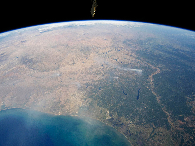
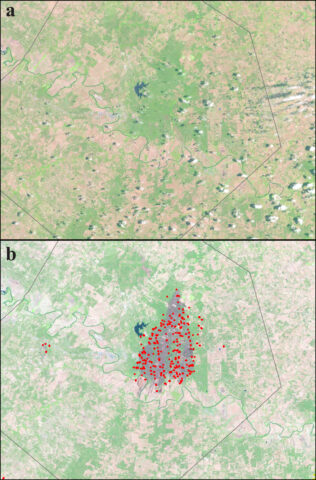
Exercise 2, “Exploring Spatial Data,” explores the 2012 drought in Texas and highlights the ability of GIS tools to combine several spatial data sets in one application. Figure 1 illustrates how satellite imagery from different sources can be used to analyze wildfires in a GIS framework. This exercise integrates data from the U.S. Drought Monitor, station-based meteorological data, Landsat remote sensing observations, Moderate Resolution Imaging Spectroradiometer (MODIS) fire locations, and land use data sets to better understand how drought affects wildfires.
Exercise 3, “Data Symbology and Classification,” analyzes the official hurricane track for Hurricane Sandy, along with the Federal Emergency Management Agency’s Impacts Database. The combination of these two data sets allows students to create a map that helps to better communicate the impacts from Hurricane Sandy.
Exercise 4, “Cartographic Mapping,” uses NOAA Cooperative Observer Network data to map the 1993 blizzard, often called the Superstorm, that dumped record snowfalls over much of the East Coast of the United States. An illustration of this mapping exercise in shown in Figure 2.

Finally, Exercise 5, “Coordinate Systems and Map Projections,” explores map projections and datum concepts using climate model simulation output provided by NOAA and the U.S. Global Change Research Program.
Future Work
In 2016, the “GIS Tutorial for Atmospheric Sciences” will be expanded to include additional exercises that focus on intermediate and advanced topics in GIS. This new section will teach students about working with netCDF in ArcMap, analysis and geoprocessing tools, Web mapping, and animation of data through time. In addition, we plan to develop a version of the tutorial that will be based on the Quantum GIS (QGIS) open-source GIS platform. Feedback from students, educators, researchers, and practitioners will guide the development of new hands-on exercises that integrate atmospheric sciences with GIS tools and methods.
References
Armstrong, L., K. Butler, J. Settelmaier, T. Vance, and O. Wilhelmi (Eds.) (2015), Mapping and Modeling Weather and Climate with GIS, Esri Press, Redlands, Calif.
Bolstad, P. (2005), GIS Fundamentals: A First Text on Geographic Information Systems, XanEdu, Ann Arbor, Mich.
Cutter, S. L. (2003), GI science, disasters, and emergency management, Trans. GIS, 7(4), 439–446.
Miller, R. W., R. J. Hauer, and L. P. Werner (2015). Urban Forestry: Planning and Managing Urban Greenspaces, Waveland, Long Grove, Ill.
Taramelli, A., E. Valentini, and S. Sterlacchini (2015), A GIS-based approach for hurricane hazard and vulnerability assessment in the Cayman Islands, Ocean Coastal Manage., 108, 116–130.
Uejio, C. K., O. V. Wilhelmi, J. S. Golden, D. M. Mills, S. P. Gulino, and J. P. Samenow (2011), Intra-urban societal vulnerability to extreme heat: The role of heat exposure and the built environment, socioeconomics, and neighborhood stability, Health Place, 17(2), 498–507.
Waters, K., et al. (2005), Polygon weather warnings—A new approach for the National Weather Service, paper presented at the 21st International Conference on Interactive Information Processing Systems (IIPS) for Meteorology, Oceanography, and Hydrology, American Meteorological Society Annual Meeting, San Diego, Calif.
Wilhelmi, O. V., and T. L. Betancourt (2005), Evolution of NCAR’s GIS Initiative: Demonstration of GIS Interoperability, Bull. Am. Meteorol. Soc., 86, 176–178.
Wilhelmi, O. V., and J. C. Brunskill (2003), Geographic information systems in weather, climate, and impacts, Bull. Am. Meteorol. Soc., 84, 1409–1414.
Wilhelmi, O. V., and R. E. Morss (2012), Integrated analysis of societal vulnerability in an extreme precipitation event: A Fort Collins case study, Environ. Sci. Policy, 26, 49–62, doi:10.1016/j.envsci.2012.07.005.
Author Information
Jennifer Boehnert, National Center for Atmospheric Research, Boulder, Colo.; email: [email protected]; J. Greg Dobson, National Environmental Modeling and Analysis Center, University of North Carolina at Asheville, Asheville; and Olga Wilhelmi, National Center for Atmospheric Research, Boulder, Colo.
Citation: Boehnert, J., J. G. Dobson, and O. Wilhelmi (2016), Teaching the integration of geography and atmospheric sciences, Eos, 97, doi:10.1029/2016EO046011. Published on 25 February 2016.
Text © 2016. The authors. CC BY-NC 3.0
Except where otherwise noted, images are subject to copyright. Any reuse without express permission from the copyright owner is prohibited.