If you could fly around your research results in three dimensions, wouldn’t you like to do it? Visualizing research results properly during scientific presentations already does half the job of informing the public on the geographic framework of your research. Many scientists use Google Earth™ mapping service (V7.1.2.2041) because it’s a great interactive mapping tool for assigning geographic coordinates to individual data points, localizing a research area, and draping maps of results over Earth’s surface for displaying the results in three dimensions. Yet scientists often do not fully explore the Google Earth™ platform.
Visualizations of research results in vertical cross sections through these maps are often not shown at the same time as the maps. However, a few tutorials to display cross-sectional data in Google Earth™ do exist, and the workflow is rather simple. By importing cross-sectional data into in the open software SketchUp Make [Trimble Navigation Limited, 2016], any spatial model displaying research results can be exported to a vertical figure in Google Earth™. Here I explain an easy workflow, give some tips, and discuss some of the endless applications of the method. This workflow will give your research results better spatial visibility and allows more dynamic scientific presentations.
What You’ll Need
The only programs necessary to display results are the open software three-dimensional (3-D) drawing tool SketchUp Make and Google Earth™. Sketchup Make is mostly used for creating representations of buildings in three dimensions that can be explored in Google Earth™ when the 3-D building layer is toggled on.
Any spatial model displaying research results can be exported to a vertical figure to enable the results to be visualized spatially.
By importing a cross section into SketchUp Make, any spatial model displaying research results can be exported to a vertical figure in Google Earth™ to enable the results to be visualized spatially. These representations are, for instance, used by NASA to plot cloud formations above Earth [Chen et al., 2009]. The usefulness of the proposed workflow in this short tutorial lies in its simplicity. No external scripts linked to any specific programming language are needed.
How to Do It
For maximum visibility, the Portable Network Graphics (PNG) picture format is preferable for your figure. This format allows the background of the vertical cross section to be transparent, which is far more useful than the white background in JPEG or other formats.
The workflow is as follows (a more complete description is available in the video tutorial below, and the Google Earth™ image example described below is available here):
![Fig. 1. Five-step workflow for setting up and exporting a vertical cross section from SketchUp Make into Google Earth. Example shows a 30-km-long, NW-SE geological cross section through the North Eifel mountains in Germany [Van Noten et al., 2011]. Source: “NW Eifel” NW coordinates = 50.6166°N, 6.2511°E; SE coordinates = 50.3982°N, 6.5001°E. Google Earth. Satellite photo taken 2 August 2007. Image captured 7 July 2015. Eye altitude 2.21 km. DigitalGlobe 2015.](https://eos.org/wp-content/uploads/2016/01/15-0351_VanNoten-F01_Web-480x404.jpg)
Import the figure into SketchUp Make under File/Import and drag it vertically (parallel to the z axis, shown in Figure 1).
Exporting and Saving the Model
The downside of this method is that Google Earth™ can only handle one preview export from Sketchup at a time because the preview model will always end up in the same SUPreview0 in Google Earth™. This might be annoying for the user because new uploads from Sketchup will overwrite previous exported figures, even when the model was saved in the My Places layer in Google Earth™ and even if the layer was renamed.
Overwriting cannot occur if the model is exported or saved to a KMZ file extension, i.e., the Google Earth™ placemark file. Once a satisfactory result has been reached, it is advisable to either export the 3-D model to a KMZ file in Sketchup (if this was your last step) or save your model to a KMZ file in Google Earth™ (if your last step was to change the orientation of the profile via the properties of the model). Reopening the KMZ file from your computer’s file directory will show your results properly, and you can drag your model to the My Places folder in Google Earth™.
Some Words of Advice
If a vertical exaggeration (e.g., factor 2) is to be used in Google Earth™, this has to be taken into account when positioning the model. Exaggeration of high-relief areas might render the model invisible in Google Earth™, as your model will be situated below the exaggerated topography. An easy solution to account for this problem is to move (Tools/Move) the model in SketchUp along the z axis until it appears in Google Earth™ by moving back and forth between the two programs or by modifying the height of the model via the properties of the SUPreview0 model in Google Earth™.
Use caution when applying the method for displaying very deep cross sections, e.g., several hundreds of kilometers to demonstrate crustal changes in Earth. If the vertical scale is too large, one may visually lose the connection with Earth’s surface. Rescaling the z axis of the figure would then be the best way to show results properly.
Cross-sectional data are meant to interpret Earth’s structure. Unfortunately, Google Earth™ does not allow users to “cut” parts out of Earth to place your cross section “in” Earth to show crustal properties of inner Earth. This might be a new tool in the future, but for now, the proposed visualization tool is the best solution geologists have.
Applicability
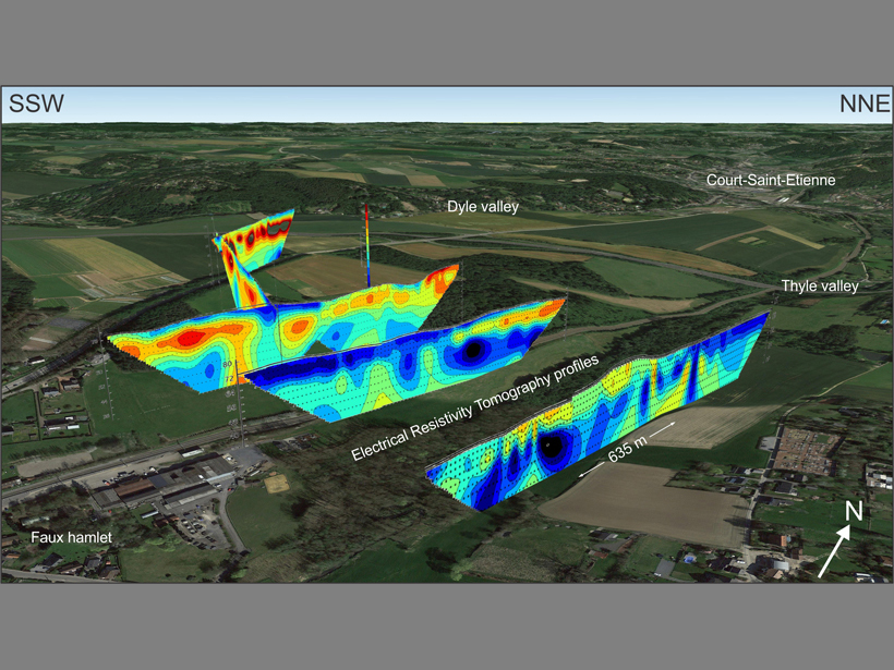
Although this workflow demonstrates how one vertical cross section can be displayed, the applications of visualizing results are endless.
Although this workflow demonstrates how one vertical cross section can be displayed, the applications of visualizing results by using SketchUp Make are endless. Instead of importing one rectangular profile, one can easily import numerous parallel and crossing figures to create a semi-3-D effect (e.g., the image at the beginning of this article), a circular model, or any random figure fitting the representation of the research results.
Models can also be rotated along the horizontal axis to display changes, e.g., along valley or volcano flanks. For large global representations, figures might need to be separated into several parts or curved to account for the curvature of Earth (Figure 2).
![Fig. 2. Example of a crustal-scale model adapted to the curvature of Earth showing a semi-3-D representation of lithospheric layering in the North American Craton (data from Yuan and Romanowicz [2010]). Credit: Nature Publishing Group (used with permission)](https://eos.org/wp-content/uploads/2016/01/15-0351_VanNoten-F02_Web-480x270.jpg)
This visualization tool does not need to be restricted to geology. Photographs or any parameter that varies with distance can be represented vertically. Once your model is exported to Google Earth™, you can fly around it, export the various views, or make a fly-through movie and impress your audience during your next conference presentation.
Acknowledgments
The editors, an anonymous reviewer, M. E. Cushing, and M. Van Camp are thanked for their suggestions on the paper. T. Lecocq, J. Molron, A. Watlet, and A. Triantafyllou are acknowledged for testing the workflow. K.V.N. is supported by the Fonds de la Recherche Scientifique (Belgium) under grant PDR T.0116.14.
References
Chen, A., G. Leptoukh, S. Kempler, C. Lynnes, A. Savtchenko, D. Nadeau, and J. Farley (2009), Visualization of A-Train vertical profiles using Google Earth, Comput. Geosci., 35, 419–427.
Trimble Navigation Limited (2016), SketchUp Make, Sunnyvale, Calif. [Available at https://www.sketchup.com/products/sketchup-make.]
Van Noten, K., P. Muchez, and M. Sintubin (2011), Stress-state evolution of the brittle upper crust during compressional tectonic inversion as defined by successive quartz vein types (High-Ardenne slate belt, Germany), J. Geol. Soc. London, 168, 407–422.
Van Noten, K., T. Lecocq, A. K. Shah, and T. Camelbeeck (2015), Seismotectonic significance of the 2008–2010 Walloon Brabant seismic swarm in the Brabant Massif (Belgium), Tectonophysics, 656, 20–38.
Yuan, H., and B. Romanowicz (2010), Lithosperic layering in the North American Craton, Nature, 466, 1063–1068.
Author Information
Koen Van Noten, Seismology-Gravimetry Section, Royal Observatory of Belgium, Brussels, Belgium; email: [email protected]
Citation: Van Noten, K. (2016), Visualizing cross-sectional data in a real-world context, Eos, 97, doi:10.1029/2016EO044499. Published on 2 February 2016.
Text © 2016. The authors. CC BY-NC 3.0
Except where otherwise noted, images are subject to copyright. Any reuse without express permission from the copyright owner is prohibited.